
…does not exist.
At least, I couldn’t manage. The requirement of a specific and large number of spacetime dimensions (26 for the simpler bosonic string theory, 10 for the more sophisticated superstrings) is one of the most misunderstood aspects of the theory and definitely the essential ingredient for the majority of negative gut feelings towards it. It seems like there should be more effort from string peeps to explain in the simplest way possible the origin of these bizarre numbers to non-experts.
To be more specific, the real magical number is not the dimension \(D\) itself of spacetime, but \(D-2\), the number of dimensions transverse to the string, the ones it can oscillate into (minus one for the time dimension, and minus one for the dimension longitudinal to the string). In other words, the 1D string traces a 2D surface in spacetime, called a worldsheet. The magic number is the number of remaining directions available to the string, so \(D-2\).

This picture has been badly drawn at least one thousand times, but I felt like badly drawing it yet one more time.
Thus the magic number is 24 (or 8 for the superstring). 24 is truly a mystical number. John Baez provides a fantastic account of why 24 is his favourite number, hinting at scattered mathematical gems in which it makes unexpected appearances. Some of them look like absolutely nothing else than pure numerology:
and this only works for \(24\), except 0 and 1 of course. (If you like tough math puzzles, try proving this. I don’t). It is nothing else than incredible that this funny identity is related to unexpectedly complex and fascinating mathematics (monstrous moonshine), and string theory (which acts as the “glue” that brings together monstrous moonshine). Also relevant is the appearance of 24/2 in the crazy series
In fact, that is why in bosonic string theory \(D-2 = 24\). In superstrings, the equivalent madness is
which gives \(D-2 = 8\). You should at this point be convinced that I’ve lost it completely. After all, these sound like random unrelated facts (and “facts”) and even though each one of them could be easily explained to a layman, I’m not really explaining what the relationship should be with the number of dimensions in string theory. I sound mad not because I say things that are wrong, but because these things are incoherent and disconnected. The problem is that the connective tissue is too technical, either mathematically, or physically, or stringly, for me to explain simply.
How to convince someone that \(D-2 = 24\) with the least effort possible? It’s much easier if they accept the crazy equation \(1+2+3+\ldots = -1/12\); but that’s clearly not satisfyingly rigorous. Even if it is possible to make sense of it, for example, with ζ-regularization, aka with heat-kernel regularization + analytic renormalization (and there is already a lot of material on this around) this would still be unsatisfactory, since there is no non-shady reason for which all of this manipulation should have anything to do with the physics. Is it possible to arrive to the correct results without this crazy equation; actually, without ever encountering any “irregularity” to regularize? Yes, sure. But exactly how brief and elementary can we be doing that?
I’ve found that proofs of \(D=26\) can be classified roughly as such:
- Light-cone quantization
- with crazy eqt. Requires a bit of knowledge about the polarizations of massive/massless vector bosons.
- without crazy eqt. Requires essentially studying all of the string’s quantization / Virasoro algebra.
- Conformal field theory
- without crazy eqt. Requires knowing conformal field theories and conformal anomalies.
- Modular invariance
- with crazy eqt. Requires fairly elementary QM and math.
- without crazy eqt. Requires elementary QM but an f-ton of basic, but tedious complex analysis.
Proof 1.1, I’ve done it here a while ago. It’s pretty easy, but you need to trust the crazy equation. The other proof with the crazy equation, 3.1, is in Baez’s slides.
The crazy-free proofs curiously form an unholy trinity. Each only requires knowledge from one vertex of a triangle spanning between
- String theory
- Theoretical physics
- Mathematics
for a certain (surely biased) interpretation of these terms. Proof 1.2 is the most common in introductory string theory, since you’re already learning the necessary string physics anyway, and it’s mathematically not intimidating. Proof 2.1 is for a more advanced study and gives a very clear physical interpretation of the critical number of dimensions as it is directly related to the cancellation of a conformal anomaly. Proof 3.2 I’ve never seen before - it seems ideal for people that know some basic complex analysis (residue theorem is all we need) and some really basic quantum mechanics, and requires next-to-no knowledge about string physics.
I’ve tried really hard to squeeze an easy proof that is “rigorous” (doesn’t use the crazy equation), but I have failed. I have come to believe the three vertices of the triangle are to be understood as translation in different languages of the same conceptual core, and that core is irreducible. So if two of the links in the chain are brought to a minimum complexity, the third has to eat it all up.
All I could manage is the following realization of proof 3.2. This will bring the theoretical and string physics to the background and will concentrate on the mathematics, and will be as rigorous as possible on the mathematical side (while occasionally being slightly handwavy on the physics). It turns out quite longer than what you would call elementary, but I find it satisfying that it builds the number 24 piece by piece (as 2, times 3, times 4). Consider it a letter of apology for releasing \(1+2+3+\ldots=-1/12\) into the wild; if you care, here it is.
The proof
We have already talked about the worldsheet, the surface the string traces in spacetime. On this surface, we can set up a coordinate system \((\sigma^1,\sigma^2)\). Clearly, it is sensible physically that while observables might be written in terms of these coordinates, they should be invariant under coordinate changes \((\sigma^1,\sigma^2) \rightarrow (\sigma^{1}\prime,\sigma^2 \prime)\). After all, the coordinates are arbitrary to begin with. A simple example of (local) coordinate change is a dilation/rescaling: \( \renewcommand{\Re}{\operatorname{Re}} \renewcommand{\Im}{\operatorname{Im}}\)
so we understand that our theory’s observables must be invariant under such rescalings. This is easy to do classically, but becomes highly non-trivial when the thing becomes quantum-mechanical. This scale symmetry is part of the so-called worldsheet conformal symmetry of string theory.
Imagine a situation in which a string loops in time to trace a torus in spacetime. Surely, a lot of possible tori shapes are all equally valid choices. We want to compute the probability for this process to happen with a specific torus shape, or better the quantum amplitude, whose squared modulus is the probability. A basic point of quantum mechanics is that we can calculate the amplitude by summing \(\exp(i E_i t) \) over all possible states \(i\) each with energy \(E_i\), through the time passed \(t\). Thus
is the total amplitude. \(Z\) should respect our desired symmetries.
An important point is that a composite system AB of two non-interacting subsystems A and B has \(Z_{AB} = Z_A Z_B\). Because of this nice property, we can first concentrate on computing the \(Z\) of a string oscillating in one single transverse dimension, and then take that to the power of \(D-2\) to make it wiggle in \(D-2\) transverse dimensions.
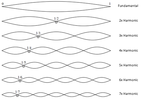
Just like actual vibrating strings, string theory strings have harmonics which are integer multiples of the fundamental.
So a string is almost exactly like an actual guitar strings and has infinite oscillation modes, or harmonics, or overtones. Each one of them is a harmonic oscillator, which in the quantum version has energy levels
Right? So the \(Z\) of one quantum harmonic oscillator is
The geometric series I just summed appears to have ratio \(|r| = 1\), which means it actually does not converge. Let’s rip off the bandaid right now: the \(Z\)s, defined naively as we did, almost never converge in a Lorentzian (i.e. spacetime) theory. Often we physicists say they are “oscillatory” because we sum a bunch of \(exp(ix)\) factors, and then handwave that they somehow magically cancel, but this is a cheap lie - we just mean they don’t converge. This is true not just in string theory but in all of quantum field theory, or standard quantum mechanics, or even the lowly quantum harmonic oscillator.
How can we move forward? The correct way to do it (and to word it) with is to make time a complex variable. By giving it an imaginary part, these \(Z\)s are made to converge. Not only: when you compute directly observable quantities from this, and then take \(t\) back to the real axis, you recover sensible answers (which match experiment when possible). So, this is not a trick; this prescription is our definition of what it means to have a quantum theory in spacetime.
tl;dr: don’t worry, assume \(t\) is complex and in the upper half-plane \(\Im t > 0 \).
To get back on track, we had that one string in one dimension had infinite oscillation modes, which clearly have frequencies which are integer multiples of the fundamental. In fact, \(\omega = 1,2,3,\ldots\) and so the \(Z\) for our 1D string is the product
…and we fell off the deep end. The madness of \(1+2+3+\ldots\) catched up with us. If we were weak in spirit, we would succumb and substitute \(1+2+3+\ldots \rightarrow - 1/12\), and we would get the correct answer, skipping almost all of the math in this article. But we are not here for this, we are here to make that \(24\) come out without using witchcraft. Therefore, let’s proceed.
Why did that divergent sum appear in that exponent in the first place? If you trace our calculations back it comes from the zero-point energies of the QHOs, the \(E_0 = \frac{\omega}{2}\). However, zero-point energies are arbitrary, and that one was just a useful conventional choice. Ultimately there is an ambiguity in building a quantum HO from a classical HO called an ordering ambiguity, since you need to convert commuting variables \(p,q\) into non-commuting operators \(\hat p, \hat q\) and there is no preferential “quantization” of things like \(pq\). Is the quantization \(\hat p \hat q\)? Or is it \(\hat q \hat p\)? The difference is a constant, an arbitrariness in the zero-point energy. Thus our most conservative bet is that the ZPOs here actually sum to a finite, but unknown value:
where \(r\) is an unknown real number. Note that the mad calculation would give the magic value \(r = 1/24\). So, for my next two tricks:
- I am going to show, using a symmetry, that \(1/r\) is the number of transverse dimensions.
- I am going to show, using another symmetry, that \(r = 1/24\) anyway, even without \(1+2+3+\ldots = - 1/12\)
To start talking about these symmetries, I need to relate my variable \(t\) to the shape of the torus. The relationship is that the torus is built by gluing same-colour edges in this parallelogram:
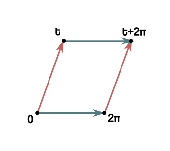
where \(t\) is represented as a point in the complex plane. (The \(2\pi\) side is the consequence of a convention that made it so that the frequencies \(\omega = 1,2,3,\ldots\) were integers). Or to clean up the notation, with \(\tau = t/2\pi\) (and a simple rescaling, which I remind is a symmetry):
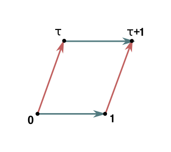
Note that when \(\tau\) moves to the real axis the torus degenerates. That makes physical sense: can a string really loop back unto itself in real time? That’d be time travel. It can only happen in imaginary time or at least in the upper half-plane.
Defining \(q := e^{i 2\pi \tau}\), our \(Z_{1,L}\) becomes
First trick
First of all, if we shift \(\tau \rightarrow \tau + 1\), we get different parallelograms:
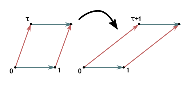
but they make the same torus after gluing (check it!). If the shape does not actually change, then the physical quantities shouldn’t either.
However, under this transformation our amplitude does transform:
That makes no sense… until we remember that this is only for one dimension. For \(D-2\) transverse dimensions, the total amplitude is \(Z_{1,L}^{D-2} \), which will remain invariant if
this equation defines the critical dimension of the string theory. If we will find an integer value of \(1/r\), then the theory will make sense only in \(D = 1/r + 2\) spacetime dimensions.
Now, proving that \(r = 1/24\) will not be as easy. Let’s try.
Second trick
The other symmetry we will consider is to send \(\tau \rightarrow - 1/\tau\). The resulting tori are not identical but they are similar - they are rescaled versions of eachother. You can check that the original \(1\) side matches with the new \(-1/\tau\) side and the original \(\tau\) side matches with the new \(1\) side. As we said, rescalings of the worldsheet should be a symmetry.
Thus the total amplitude must be invariant under this; however we should not expect \(Z_{1,L}^{D-2}\) to necessarily also be. Huh? Wasn’t \(Z_{1,L}^{D-2}\) the total amplitude? No, I lied to protect you from the harsh truth. The truth (part of it) is that oscillation on a string always come in pairs. There are many possible characterizations of this dichotomy: left-movers and right-movers, holomorphic and antiholomorphic, sine and cosine…
What matters is that to our \(Z_{1,L}\) (the \(L\) is now understood to stand for “left”) there will also be a paired \(Z_{1,R}\) for the sister oscillations. Thankfully, I’ll just handwave that \(Z_{1,R} = Z_{1,L}^* \) so that the overall amplitude is the product \(|Z_{1,L}^{D-2}|^2\).
However, that is still not all: while we have accounted for oscillations of the string about a “reference” position, we also need to account for the overall movement of the centre of mass in space. We want the string to be back to its original point after time \(\tau\) if we want it to loop into a torus; but we cannot just want it, we need to include the probability amplitude for it to happen.
What is the probability amplitude for a quantum particle in 1D to stay in the same place after a certain amount of time? A hint is that for purely imaginary times, the Schroedinger equation is the heat equation. And an infinitely concentrated speck of heat evolves under the heat equation in 1D by spreading into a gaussian whose peak decreases as \((\operatorname{time})^{-1/2} \). Thus, let me guess the amplitude for the centre of mass is something like this
If so, putting everything back together the total amplitude should be something like
Ok, now under \(\tau \rightarrow -1/\tau\),
therefore if \(Z_{1,L}\) were to transform in some way similar to this:
our total amplitude would be invariant, and our theory would make sense. I’m now set to prove that this can only happen if \(r=1/24\).
Sorcery
Let’s do some preliminary rewriting.
Then, a more comfortable presentation of the product \(P(\tau)\):
I’ve used the Taylor expansion for \(-\log(1-x) \) and the geometric series. If you are not convinced, you can check more carefully these steps (including the sum swap) are sensible for \(\Im \tau > 0\).
Now:
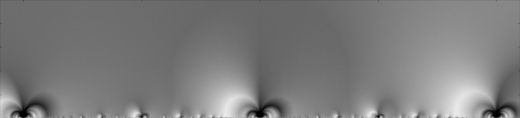
The following psychedelic argument is due to Siegel (yeah, that Siegel). We start for no apparent reason from this function of a complex variable \(w\), with \(\tau\) as a parameter:
and then, introducing another real parameter \(\nu\) (our finishing move will be to send this to infinity), we construct the combination
Let’s count the poles of \(g\). A quick inspection shows there is a set of simple poles at \(w = \pm \frac{\pi k}{\nu}\) and another at \(w = \pm \frac{\pi k \tau}{\nu} \), for \(k = 1, 2, 3, \ldots\); plus a triple pole at \(w = 0\). The residues are easily computed as follow:
If the residue at the triple point doesn’t seem obvious, recall that the Taylor expansion of the cotangent at zero starts \(\cot s \sim \frac{1}{s} - \frac{s}{3} \).
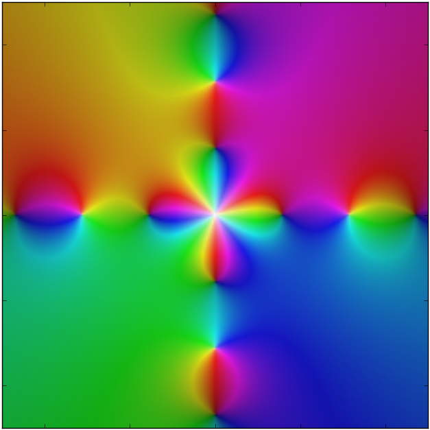
Colour wheel plot of (g(w)), for (\tau = i), (\nu = 1). The white specks are the poles, and the order is how many times the colours repeat circling them.
Now, it should be clear the intention is to exploit \(g\) for an application of the residue theorem. We consider the path \(\gamma\) running ccw around the parallelogram with vertices \(1,\tau,-1,-\tau\).
The residue theorem says
The sum is actually only over those poles that are inside the parallelogram, but we’ll see in a little while that’s not something we should worry about.
Now, I would like to use this equation to prove the identity we actually need. I will only prove it, however, for \(\tau\) on the imaginary axis, because it’s simpler, but it will actually be true for all \(\Im \tau > 0\). Since both sides of the equation I’ll derive are holomorphic in \(\tau\) over the upper half-plane, them agreeing on a line is enough to prove they are always equal. Long story short: assume \(\tau\) is purely imaginary for now, but at the end we can just drop this assumption.
Let’s do the integral on the parallelogram, which is now a rhombus. \(g(w) = f(\nu w) w^{-1} \) doesn’t seem to be an easy function to guess an antiderivative for. So let’s take the \(\nu \rightarrow \infty\) limit. It’s not hard to see that \( f(\nu w) \) converges to the constant \((1,-1,1,-1)\) respectively on the four segments of \(\gamma\) (if you don’t see it, write \(\cot s\) using complex exponentials). Thus in the limit the integral is
Easy! The integral of \(1/w\) is \(\log w\), so let me just plug that in and… aaagh! Branches! We need to choose a branch for the log, and make sure the path does not jump over the branch cut. We can use symmetry to rewrite
and now that the path is all on the right, we can use the negative real axis as a branch cut and thus use the principal branch of the logarithm. Keeping track of everything at the end you get
Nice. Now for the residues. If \(\nu \rightarrow \infty\), all the poles shrink and move closer to the origin; so in the limit they are all inside the rhombus and the sum is over all poles. Thus the sum is
Note
plug that in, and you’ll recognize that the sum of the residues becomes
Finally we’re starting to get back to Earth. This is starting to look like a theorem about our \(P(\tau)\) product. Now that we have LHS and RHS, let’s use the residue theorem.
There’s our magic number! Half of it at least. This still looks like gibberish though… let’s exponentiate for good measure:
This seems not much of a fact about \(P(\tau)\), but about the combination
which we just proved transforms “nicely” under a \(\tau \rightarrow - 1/\tau\) transformation:
And that’s it! That’s what we were looking for. For \(Z_{1,L}^{-1}(\tau)\) to transform how we want, it has to be \(\eta(\tau)\) itself, and so \(r=1/24\), and so, finally
Conclusions
Because of the philosophy behind this whole post, to only use mathematics as elementary as possible and to have it be self-contained, we sped by what is actually incredibly fascinating (and surely much more elegant) math. \(\eta(\tau)\) is, of course, the Dedekind eta function, and what we proved are its transformation properties under the modular group; more precisely that the modular discriminant \(\Delta(\tau) := (2\pi)^{12} \eta^{24}\) is a modular form of weight 12. String theory is tightly connected to this area of mathematics; in fact I hope that for those that already know this stuff this served as a sneak peek of what strings even have to do with modular forms. Anyways, I don’t think I would do justice to a subject I actually barely know the basics of, so I’ll shut up now.
An interesting question that pops up sometimes: if it’s so wrong, why does \(1+2+3+\ldots = -1/12\), or ζ-regularization / heat kernel / Abel summation or whatever you want to call it, give the same correct result as more rigorous paths, with one tenth of the effort?
I have no idea.
Instinctively I would babble something about “physically reasonable” or “analyticity” but frankly this is just pure madness. It’s definitely not a coincidence because the same trick works for superstrings too. In fact I’m not even sure what the exact relationship between the three different classes of proofs are, they look like completely different reasonings. In light-cone quantization, on a first reading you don’t even realize how the scale/conformal invariance even fits in - it’s very hidden. And if you happen to know some conformal field theory, go take a look at how that proof builds the 24. They don’t sound exactly like translations of the same thing, even though they have to be.
It’s fascinating how much information about the content of the theory the proofs of \(D = 26\) (or \(D=10\)) carry, and how much you already learn about strings just by trying to explain what is essentially the most basic fact about the theory. It is a limpid example of the fact that in string theory everything fits, nothing is just thrown there, everything is essential.
Addendum
There is perhaps a faster proof if you assume Euler’s pentagonal number theorem
If you complete the square in the exponent you can rewrite
thus
With \(\eta\) in this form, it is doable to prove \(\eta(-1/\tau) = \sqrt{\tau/i} \eta(\tau) \) using Poisson resummation.
Still, invoking Euler’s theorem seems definitely like cheating, so I didn’t pursue this path.
Refs
Baez, J. (2008). My favourite number: 24. Talk at the University of Glasgow.
Siegel, C. (1954). A simple proof of η(-1/τ)=η(τ)√τ/i. Mathematika, 1(1), 4-4. doi:10.1112/S0025579300000462