Solutions
Week 1
Easy
First point is dead easy. The two graphs are the same!


The above animations are by u/HarryPotter5777 and u/OnyxIonVortex.
The isomorphism is clear if you number the nodes in the left graph clockwise 1 to 7. The graph is composed of the edges of the external heptagon plus the heptagonal star inside. So you redraw your vertices in a circle, but in the order in which they appear in the star, so for example 1-5-2-6-3-7-4. Therefore the star on the left has now become the external heptagon on the right; to account for the heptagon on the left you then just connect your new numbered vertices as 1-2, 2-3, etc and you will see that you've just drawn the other heptagonal star.
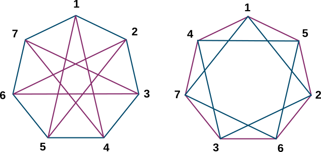
The two coloured cycles turn into eachother.
Second point is trickier. It's not hard, but it's very boring unless you have a trick.
Sure you can just compute the resistance by brute force using the normal reduction algorithm. This should give you the correct answer, \(R = 40/91 \Omega\). I haven't done this. There's a different way which makes it a bit quicker.
All quantities are in SI units, \(\Omega\), \(A\), \(V\). So I'm going to freely omit units for the sake of the math.
Consider the left graph. Forget for a moment about nodes 1 and 2 and just imagine doing this: plug current \(1A\) into node 1 and pull current \(\frac{1}{6} A\) from all the other nodes.
Now new symmetries pop up. For example, mirror symmetry about the vertical axis. This means for example that nodes 5 and 4 must have the same potential. Therefore no current flows between the resistor connecting them; in fact for the purpose of this imaginary situation the resistor can be removed and the nodes 5 and 4 identified. Same for the pairs 72 and 36. This gives us the following simplified graph:
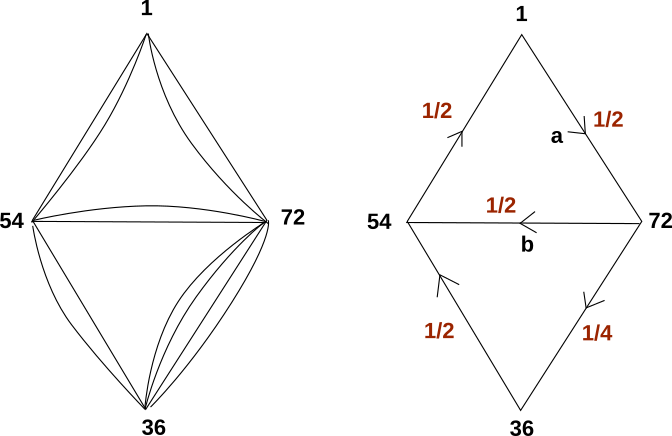
The resistances are in red, the arrow represent my choice of direction for writing signed currents.
On the right I replaced \(N\) \(1\Omega\) resistors in parallel with the equivalent \(1/N \; \Omega\) resistor just for clarity, but we need to rememeber these are actually \(N\) resistors.
So how much current actually flows in these resistors? I've named the total current flowing between 1 and 72 as \(a\), and between 72 and 54 as \(b\). We know 36, 54, 72 all pull \(-\frac{1}{3} A\) each (two \(1/6\) from each original node) while 1 gets \(+1A\). This means we know all of the other currents by current conservation. In particular it's obvious that following the square 1-72-36-54-1 the currents are
\[a, a-\frac{1}{3} - b, a - \frac{2}{3} - b, a - 1\]
Now that we know the current except for the variables \(a\) and \(b\), let's find \(a\) and \(b\). We know in a loop the total potential drop (sum of currents times resistances) must be zero. Taking as loop the upper triangle, we get
\[\frac{1}{2} \left( a + b + a - 1 \right) = 0 \Rightarrow b = 1-2a\]
That's cool. We need two loops to fix two variables though; a nice second loop is the external square. This gives (multiplying it all by \(2\) in advance):
\[a + \frac{1}{2} (a - \frac{1}{3} - b) + (a - \frac{2}{3} - b) + a - 1 = 0\]
\[\Rightarrow a = \frac{20}{3\cdot 13}\]
Where I've used the previous relationship with \(b\).
The reason for all of this dance we're performing is we want the voltage between 1 and 2 which is the one between 1 and 72 of course. But this is just the current flowing in the 1-72 resistor, times its resistance. So
\[V_{1-2} = \frac{1}{2} \frac{20}{3\cdot 13} = \frac{10}{3\cdot 13}\]
Surprisingly, that's all we need to solve the original problem. Basically, we inserted \(1A\) in node 1 and \(-\frac{1}{6} A\) in all the others, and obtained a potential difference \(V_{1-2}\) between nodes 1 and 2. We can imagine instead inserting \(1A\) in node 2, and \(\frac{1}{6} A\) from all the others; by symmetry we will obtain a potential difference \(-V_{1-2}\) between 2 and 1, aka \(V_{1-2}\) again between 1 and 2.
We can superimpose these situations! This stuff is linear. We sum the currents and the voltages. The total current entering 1 is \(1 + \frac{1}{6} A = \frac{7}{6} A\) and the one exiting 2 is also \(\frac{7}{6} A\). The current entering the nodes 3-7 cancels in the sum. So in this summed situation we're exclusively passing current from node 1 to 2. Moreover, the sum potential between 1 and 2 is \(2 V_{1-2}\).
So the total resistance between 1 and 2 is:
\[R = (2 V_{1-2}) / (\frac{7}{6} A) = \frac{20}{3\cdot 13} \cdot \frac{6}{7} = \frac{40}{91}\]
Ok, that wasn't exactly straightforward. But I think it's significantly faster than brute-forcing through it.
Hard
I'm gonna set \(c=1\) and signature \((+,-,-,-)\).
The premise of the problem should make you suspicious a little. The ships performs \(7\) left turns of \(\pi/2\) each, but in the end it has the same orientation, meaning it has performed a full turn of \(2\pi\) (a priori it could have done any integer number of full turns, but we will prove at the end that more than one turn doesn't work). \(\frac{7}{2}\pi \neq 2\pi\) so something isn't right.
The thing is that in relativity when something accelerates, and the acceleration is not parallel to its velocity, it also rotates a bit. This is called Thomas precession, and it boils down to boosts not commuting. The commutator of two small boosts in the x and y direction for example is a small rotation about the z axis.
This makes things very complex. As the ship accelerates in each segments, it is slowly rotating. The acceleration itself is directed towards its front and so this gets messy. On average over the whole cycle the Thomas precession will have made the ship rotate right so that combined with the ship's turns the total angle is \(2\pi\).
There's a way to recast this thing into very simple geometric language in which it becomes almost stupidly easy.
Remember that four-acceleration is \(A^\mu = \frac{dU^\mu}{d\tau}\). Squaring
\[dU^\mu dU_{\mu} = a^2 d\tau^2\]
Where \(a^2 = A^\mu A_\mu\) is the proper acceleration. The above equation means that if we take \(dl^2 = dU^\mu dU_{\mu}\) as a line element (a metric) on the space of 4-velocities, then a spaceship moving at constant proper acceleration is just tracing curves in 4-velocity-space at "constant speed", that is \(\tau\) is just the arc length (actually, \(\tau/a\)).
However, \(U^\mu\) does not belong to the full Minkowski space \(\mathbb{M}^{1,3}\). There's the constraint \(U^\mu U_\mu = 1\) (and obvs \(U^0 > 0\)). This fixes the 4-velocity to a one-sheeted hyperboloid (in green here):

in the figure the z direction is omitted. We won't be needing it for this problem, in fact. It's well known that this subset of Minkowski space, with the Minkowski metric restricted to it, is actually just hyperbolic space (with radius of curvature \(1\)). This is the celebrated hyperboloid model.
In our specific case we have Minkowski space \(\mathbb{M}^{1,2}\) (after omitting z) and the embedded hyperboloid has the geometry of hyperbolic 2-space, or the hyperbolic plane. In figure we have the mapping to the Poincaré disk model, which is cool and all, but we won't be needing this mapping. We'll only use the Poincaré disk for visualization purposes. In fact, we won't be needing any mapping or coordinate change at all.
So let's list the obvious and obviously cool facts here. The Lorentz group \(SO(1,2)\) acts on \(\mathbb{M}^{1,2}\) as the isometry group; translated in human Lorentz transformations preserve the metric \(dl^2\); so the same must be true for the hyperboloid, given that it is invariant under the transformations (the constraint is preserved) and it inherits \(dl^2\) as metric. So \(SO(1,2)\) is the symmetry group of the hyperbolic plane. (Give or take a few quotients but those are not important for this).
Different characterizations of this group can be given by considering different models. The half-plane model evidences it as \(PSL(2,\mathbb{R})\), the Poincaré disk as the disk's automorphism group. They're all the same thing.
The correspondence between the symmetries acting on the hyperboloid and on the Poincaré disk, just for visualization purposes, is as such: the two boosts in the \(x\) and \(y\) directions are the two translations, and the rotation around the \(z\) axis is the rotation of the whole disk about the centre. That's it. You can also note that just like the two boosts don't commute, neither do hyperbolic translations. Freaky stuff.
So our final goal is to compute \(\tau_{\text{total}}\), which for the above argument is the length of the path the ship traces in the 4-velocity hyperbolic plane (over \(a\)). Let's discuss the shape of this path. Let's call the instants at which the ship turns \(\pi/2\) "vertices" and the \(\tau\)-long segments "edges". We're going to see in a little while why.
Note that for any given vertex we can use a Lorentz transformation (aka an hyperbolic isometry) to the ship's instantaneous frame, where the speed at the vertex is zero, and the two edges (the directions of the ship before and after the \(\pi/2\) turn) are oriented along the \(x\) and \(y\) axes. Both of these are segments where the ship boosts starting from zero velocity and remains parallel to an axis - so they feature no Thomas rotation (in this frame) and they're simply straight. In particular, they are straight (geodesic) segments of the hyperbolic plane.
By a similar argument, using the same frame, it's very easy to show that the angle the ship turns at the vertex is exactly the hyperbolic angle between the two edges.
Since both the above points are invariant under Lorentz transformations, these hold for all of the edges and vertices independently of the frame we choose. So our path is made of straight, equal length segments, in a closed loop, all forming an equal angle with the next...
That's a regular polygon. The ship's velocity traces a regular, right-angled heptagon in the hyperbolic plane. These can tile the hyperbolic plane, with 4 at each vertex. Here's the tiling in the Poincaré disk:

All of these are identical regular right-angled heptagons. And each one of them is the trajectory of our ship in velocity-space. (Note that the Poincaré disk is a conformal model - this means the angles we see represented are the real angles).
We just need the perimeter. We work exactly like in Euclidean geometry. We draw the perpendicular to an edge of the heptagon passing through its centre, and the line from the centre to one vertex. We obtain a right triangle with angles \(\pi/2\), \(\pi/7\), and \(\pi/4\). The following theorem holds for hyperbolic right triangles:
\[\cos(\alpha) = \cosh(A) \sin(\beta)\]

where \(A\) is the length of the side opposite angle \(\alpha\), and \(\beta\) is the remaining non-right angle. Therefore the side of the triangle we care about (half the edge of the heptagon) is
\[A = \cosh^{-1}( \cos(\pi/7) / \sin(\pi/4))\]
and the total proper time is
\[7\tau = \frac{1}{a} 14 \cosh^{-1}( \sqrt 2 \cos(\pi/7))\]
And that's it. Now let's clear two side points:
- In the hint I said if you replace \(7\) with \(n\), the problem is unsolvable if \(n<4\), and the result is \(0\) if \(n=4\). This is crystalline in the formalism we've set up. A right-angled \(n\)-gon lies in the hyperbolic plane only if \(n>4\), a right-angled square is just a regular square in the Euclidean plane; and the right-angled triangle and digon are spherical polygons. The latter two are simply not possible physically in our example. The square is a boundary case; a small enough patch of hyperbolic space looks like flat space. So the right angled square exists, so to speak, in the hyperbolic plane if we send its size to zero. Physically, if \(\tau\) is so small that we are in the nonrelativistic limit throughout, velocities add linearly and there is no Thomas rotation.
- I never said the ship should make one full turn. It could have made 2, or 3, or whatever full turns to get back to its original orientation. This corresponds to considering nonconvex regular heptagons, aka heptagonal stars, aka heptagrams. There's only two possible heptagrams, and they are the ones in the Easy problem, the 7/3 and 7/2 stars, in which one spins respectively 3 or 2 full turns. These cannot be done right-angled in the hyperbolic plane, though, because they have acute angles when drawn in Euclidean space. This means they only exist as right-angled in spherical geometry. So it was just one turn after all.
Week 2
Winding rope
Angular momentum is not conserved, as the rope applies a tension on the little body that is off-axis. The tension is instead always orthogonal to the velocity of the body, so that energy is conserved. Some people might have issues figuring out intuitively why tension and velocity are normal; an easy way is to imagine the ball is a regular polygon instead of a circle, then sending the number of sides to infinity.
Anyways, the rope and the radius vector between the centre of the ball and the contact point are always orthogonal, because the rope is tangent to the ball, so that they rotate rigidly together and the angle the first make with the horizontal direction is the same the latter makes with the vertical direction; we call it \(\theta\).
As the contact point has moved an angle \(d\theta\) along the surface of the ball, a length \(Rd\theta\) of rope has deposited, so that the remaining length \(l\) of rope decreases as \(\dot l = - R \dot \theta\).
Also, since the energy and so the speed is constant and orthogonal to the rope, it's always true that \(v_0 = \dot \theta l\) because the body is performing circular motion around the contact point. This gives us an expression for \(\dot \theta\) we can substitute in the previous relationship to obtain
\[\dot l = - R v_0 / l \Rightarrow dl\,l = - R v_0 dt \Rightarrow \frac{l^2}{2} = \frac{l_0^2}{2} - R v_0 t\]
So that the time such that \(l=0\) is \(t^* = \frac{l_0^2}{2 v_0 R}\). Since the speed is constant, the total displacement is simply \(s = v_0 t\).
Note: this wasn't a hard problem per se. The interesting question is about conservation of angular momentum and energy; in particular it's interesting to argue whether instead of imagining the ball to be magically fixed in space we can approximate it by attaching it to the Earth. In practice: if we realize this experiment with an actual pole of radius \(R\) fixed in the ground, will we see conservation of energy and nonconservation of angular momentum?
Funnily enough, having the Earth have a ridiculously large mass is not enough. u/Josef--K argues that the violation of angular momentum conservation must be actually accompained by an equal and opposite amount of angular momentum provided to the Earth. Now this torque \(\tau\) will result in a change in the rotational energy of the Earth according to the rotational work-energy theorem:
\[\frac{dE_\mathrm{Earth}}{dt} = \omega_{\mathrm{Earth}} \cdot \tau\]
Where \(\omega_{\text{Earth}}\) is the Earth's angular velocity. This, by conservation of overall energy, must correspond to an energy loss in our system. Note that the energy loss does not become small in the \(M_\mathrm{Earth}/m \rightarrow \infty\) limit; in fact it's completely independent on the Earth's mass.
The point is we should take another limit, namely \(\omega_\mathrm{Earth}/\omega \rightarrow 0\) where \(\omega\) is the typical angular velocity of our ball. This is readily realized in our case as the angular velocity of the Earth is pretty small (a weird coincidence is that \(\omega_\mathrm{Earth} = 2 \pi / (1 \,\mathrm{day})\)). What is the physical relevance? What happens when this limit does not hold? In that case our system has parts rotating so slow that the Coriolis and centrifugal forces pop up.
Bubble
Some care is required for this problem. The presence of the incompressible fluid should be carefully considered. Since the fluid has negligible mass, it will not be able to store kinetic energy in its flows; this simplifies the treatment as we do not need to solve for those flow but only for the membrane's dynamics. It does not mean we can ignore the fluid. It will contribute a strong element to the dynamic of the membrane in the form of a fixed-volume constraint. This is the sense of question 1: we all know information propagates at the speed of sound in the vibrations of a usual membrane - but can some magic appear if the membrane bounds a volume which is instantaneously aware of all volume changes?
Consider an extreme case of a long cylinder bounded by two circular membranes filled with the same liquid. Striking one end of this drum transmits information instantaneously to the other drum. Something similar could happen here, right?
We study this explicitly. Let's consider the potential energy of the membrane. This will be
\[V = \tau \cdot \mathrm{Area}\]
of course. The area itself can be calculated by a variation on this formula for the area element of the graph of a function \(f(x,y)\):
\[dA = dx dy \sqrt{ 1 + |\nabla f|^2 }\]
In our case, our dynamical field is the perturbation to the radius of the bubble defined as \(r(\theta,\phi) =: R + \xi(\theta,\phi)\) and the above formula is modified for the sphere to
\[V = \tau \int d^2\Omega (R+\xi)^2 \sqrt{1 + |\nabla\xi|^2 }\]
Here, \(|\nabla\xi|^2\) must be defined through the spherical gradient as \(\frac{1}{(R+\xi)^2} (\partial_\theta \xi)^2 + \frac{1}{(R+\xi)^2 \sin^2(\theta)} (\partial_\phi \xi)^2\), though since we're working at leading order we can approximate this with the actual spherical gradient on the normal sphere, by replacing \((R+\xi)^2 \sim R^2\) in the denominators. The actual explicit form is not important, just that we can approximate the \(\nabla\) on the curved surface of the bubble with the \(\nabla\) of the equilibrium configuration.
So, with that given, the potential is
\[V = \tau \int d^2\Omega \;(R^2 + 2R\xi + \xi^2) \left(1 + \frac{1}{2}|\nabla\xi|^2 \right) + O(\xi^3)\]
\[ = \tau \int d^2\Omega\; \xi^2 + \frac{R^2}{2} |\nabla\xi|^2 + O(\xi^3)\]
I've eliminated the term linear in \(\xi\) because \(\int d^2\Omega \;\xi\) is just the change in volume from the equilibrium configuration, and we've said we have to reduce ourselves to deformations that don't change the volume. Also I've dropped the \(0\)-th order term because that's just a constant which will not contribute to the dynamics (it's just the elastic energy of the equilibrium configuration). Oh, and \(R^2 |\nabla \xi|^2\) is just \(|\nabla \xi|^2\) computed on the unit sphere, so let's just write
\[V = \tau \int d^2\Omega \; \xi^2 + \frac{1}{2}|\nabla_\mathbb{S}\xi|^2\]
What about the kinetic energy? Only motions orthogonal to the surface are to be considered, so that this is simply
\[\int R^2 d^2\Omega \; \frac{\mu}{2} \dot \xi^2\]
Finally allowing us to build a total Lagrangian functional which is the integral of a Lagrangian density:
\[L = \int d^2\Omega \; \mathcal{L}[\xi]\]
\[\mathcal{L} = \frac{R^2 \mu}{2} \dot \xi^2 - \frac{\tau}{2}|\nabla_\mathbb{S}\xi|^2 - \tau \xi^2\]
Having reduced ourselves to a Lagrangian which is the integral of a density over the (now unit) sphere, we've essentially reduced ourselves to discussing a 2D field theory of the field \(\xi\) on the sphere.
This is in fact a well-known action: it's the Klein-Gordon equation. If you don't know what that is, it doesn't matter. Let's just compute the Euler-Lagrange equations, these are
\[\frac{\partial \mathcal{L}}{\partial \dot \xi} = \frac{\partial\mathcal{L}}{\partial \xi} \Rightarrow\]
\[R^2 \mu \ddot \xi = - \tau \nabla^2_\mathbb{S} \xi + 2\tau\xi\]
That term \(2\xi\) is what distances us from the case of vibrations of a drum. It's due to the fact that vibrations of the surface of the sphere also change the radius at that point and that also affects the area; if the term wasn't there we'd just have
\[\ddot \xi = - \frac{\tau}{\mu} \nabla^2 \xi\]
which is just the wave equation on the sphere, with speed of sound \(c := \sqrt{\tau/\mu}\). But our situation is slightly different:
\[\ddot \xi = - c^2 \nabla^2 \xi + \frac{2c^2}{ R^2} \xi\]
This is a hyperbolic differential partial equation (on the surface of the sphere) and so it has a well-posed initial value problem. It's defined on a curved space (the Laplacian is curved) but that's not a problem for us since we can always get to a small enough patch and build cartesian coordinates \(x\), \(y\) there and obtain the flat-space equation. The wave equation in flat 2D space is solved by sums of plane waves moving at \(c\); in our case our equation is solved by sums of plane waves moving generally slower than \(c\), so sure \(c\) is the top speed at which information travels through vibrations. And it's \(c\) on the surface, so the lag between the two seismologists is the great circle arc length between them divided by \(c\) (proof: replace \(\nabla^2\) with \(\partial_{xx} + \partial_{yy}\) and plug \(\xi = \exp(i(-\omega t + k_x x + k_y y))\) and find the phase speed \(\omega/k\) and group speed \(\frac{d\omega}{dk}\)); no actual information seems to "shortcut" through the interior.
For the second question, let's just solve the damn equation. Considering we have a spherical laplacian on our hands, it would be stupid if we didn't expand in spherical harmonics. Spherical harmonics are a set of functions \(Y_l^m(\theta,\phi)\) parametrized by \(l=0,1,2,\ldots\) and \(m=-l,-l+1,\ldots,+l\) which are orthogonal (i.e., \(\int d^2\Omega\; Y_l^m Y_j^n = 0\) unless \(l=j\) and \(m=n\)). Also, they diagonalize the Laplacian as
\[\nabla_\mathbb{S}^2 Y_l^m = l(l+1) \, Y_l^m\]
We won't need any other properties of the harmonics. In fact, if you start writing down the explicit form you're probably overthinking it.
So we decompose our solution in spherical harmonics as
\[\xi(\theta,\phi) = \sum_l \sum_m A_l^m Y_l^m(\theta,\phi)\]
First of all, we immediately solve for the constraint \(\int d^2\Omega \; \xi = 0\). We note right away that \(Y_0^0\) is a constant over the sphere and so evidently violates the constraint (in fact this physically corresponds to the bubble uniformly changing in radius). How do we know all the other spherical harmonics do satisfy the constraint? Simple: using that \(Y_0^0\) is a constant
\[\int d^2\Omega \; Y_l^m \propto \int d^2\Omega \; Y_l^m Y_0^0 = 0\]
so that all other harmonics conserve volume.
We are ready to substitute our decomposition into the equation. We get
\[\ddot A_l^m = \frac{c^2}{R^2} \left( - l(l+1) + 2 \right) A_l^m\]
which is of the form \(\ddot y = - \omega^2 y\), from which we can read immediately the frequencies:
\[\omega_l = \frac{c}{R} \sqrt{ l(l+1) - 2 }\]
but wait... why is the \(l=1\) frequency zero? Sure, we eliminated \(l=0\), but what's wrong with \(l=1\), \(m=-1,0,1\)? It seems like this mode has \(\ddot A_1^m = 0\), meaning it does not oscillate at all.
The solution is the \(l=1\) modes are just (for small \(\xi\) at least) the rigid translations of the whole sphere in the three directions. These are formally deformations of the sphere, yes... but they don't yield a sphere with a different shape, just moved. They do not change the area and so have zero energy.
Just like the Earth does not randomly change course because of stuff happening in or inside it, so bubblequakes will not include these modes, because of conservation of linear momentum. These are the only modes where the centre of mass of the bubble moves. If you want to convince yourself of this fact, do like we did before: just find for example the \(z\) coordinate of the centre of mass by averaging the function \(z \propto \cos\theta\) over the deformed sphere, then recognize that this function is just a constant times \(Y_1^0\), and so the average is zero unless your mode is exactly \(Y_1^0\). Same for \(x\), \(y\) and (a suitable combination of) \(Y_1^1\), \(Y_1^{-1}\).
So the least possible frequency is from \(l=2\) and so it's
\[\omega_2 = 2 \frac{c}{R}\]
Maximum gravity
Let's assume our planet is axially symmetric. It's not hard to convince yourself this must be true intuitively. It's a bit nastier to prove, but let's skip that. So we have our point \(P\) at \(x=y=z=0\), with the field there pointing in the \(x\) direction, and the rest of the planet symmetric about the \(x\) axis.
Because of symmetry, the \(y\) and \(z\) components of the field vanish at \(P\), so that we only need to maximize the \(x\) component.
So each element of mass \(dm\) contributes \(\frac{G dm}{r^2} \cos\theta =: G dm f(r,\theta)\) to the \(x\)-component of the field at \(P\), where \(r\) is the distance and \(\theta\) is the angle the radius vector makes with the \(x\) axis.
Now consider the isosurfaces of \(f(r,\theta)\), that is surfaces where \(f\) takes a given constant value. On each isosurface, \(f\) is constant. These are obviously axially symmetric too.
Take any point \(G\) on the surface of the planet; compute \(f\) there and so find the corresponding isosurface. The isosurface crosses the planet's surface at \(G\) and so to the sides of \(G\) we will find points in the planet but outside the isosurface and points outside the planet but inside the isosurface. But what if we take a small mass element from one of the former points to one of the latter points? We bring it from a region of lower \(f\) to one of higher \(f\), thus increasing the gravity at \(P\). So our planet cannot be the one of maximum gravity at \(P\), unless its surface coincides with an isosurface.
So the surface of the planet has the shape given by the equation
\[f(r,\theta) = \cos\theta \, r^{-2} = a^{-2} \Rightarrow r^2 = a^2 \cos \theta\]
modulated by a constant \(a\). We note \(\cos\theta>0\) is needed, so that the planet lies all to the right of \(P\). To find \(a\), we find the total volume by integrating the volume element in polar coordinates:
\[V = \int_0^{\pi/2} d\theta \sin\theta \int_0^{a \sqrt{\cos\theta}} dr r^2 \int_0^{2\pi} d\phi\]
\[= \frac{2\pi}{3} a^3 \int_0^{\pi/2} d\theta \cos^{3/2} \theta \sin \theta = \frac{2\pi}{3} a^3 \int_0^1 dx \; x^{3/2} = \frac{4\pi}{15} a^3\]
This gives the \(a\) necessary to have a given total mass \(M\) as \(a = \left( \frac{15 M}{4\pi \rho} \right)^{1/3}\).
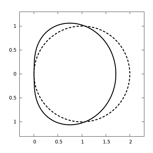
The shape of our planet compared with the sphere of equal mass (or volume). \(P\) is at \((0,0)\).
So we know our planet has the same mass (fixing density \(\rho\)) as a sphere of radius \(R = \left(\frac{V}{4\pi/3} \right)^{1/3} = 5^{-1/3} a\) (this allows us to draw the plot above); we'd like to check how much better than the sphere it performs. The field from the sphere is \(GM/R^2 = \frac{4\pi}{3} \rho G R\); while the field from our planet is the integral of \(G \rho r^{-2} \cos \theta dV\):
\[G \rho \int_0^1 d\cos\theta \int_0^{a\sqrt\cos\theta} dr\,r^2 f(r,\theta)\] \[=2\pi G \rho a \int_0^1 d\cos\theta \cos^{3/2}\theta = \frac{4\pi}{5} G\rho a\]
The ratio of the planet's field to the sphere's field is
\[\frac{g_P}{g_S} = \frac{5}{3} \frac{R}{a} = \frac{3}{5} 5^{-1/3} \sim 1.026\]
So yeah, we gained \(2.6\%\) on the field with respect to a sphere. Yay.